Full details of taking RNAseq data from Day 12 for P. helianthoides from DEG analysis, annotation, enrichment, and result figures.
Background
From the Multi-species project, I have RNAseq data from n=6 SSWD-exposed P. helianthoides and n=6 control P. helianthoides. The goal is to run a differential gene expression analysis using DESeq2 with the model of design = ~ condition, where the comparison will be between control and SSWD-exposed sea stars. Then, annotate the DEG list with gene ontology, and get enrichment using topGO with the background being all the gene ontology from all the genes from the count matrix for all P. helianthoides for the multi-species project. Then, use rrvgo and ggplot2 to make some result plots from the enrichment.
Code and output:
NOTE: Repository is still set to private until collaborators publish their genome.
github.com/grace-ac/project-pycno-multispecies-2023
Code for DESeq2 –> topGO –> rrvgo:code/43-pycno-D12-DESeq2-topGO.Rmd
Output folder: output/43-pycno-D12-DESeq2-topGO
Day 12 P. helianthoides Sample Info
Sample information:
| Individual_star_ID | sample_ID_PSC | treatment | experiment_day | bin_number |
|---|---|---|---|---|
| B9_Py92 | 522 | control | 12 | 9 |
| B10_Py86 | 528 | control | 12 | 10 |
| B11_Py81 | 534 | control | 12 | 11 |
| B12_Py85 | 540 | control | 12 | 12 |
| B14_Py94 | 552 | control | 12 | 14 |
| B16_Py95 | 564 | control | 12 | 16 |
| B1_Py89 | 519 | exposed | 12 | 1 |
| B2_Py83 | 525 | exposed | 12 | 2 |
| B3_Py91 | 531 | exposed | 12 | 3 |
| B4_Py84 | 537 | exposed | 12 | 4 |
| B6_Py87 | 549 | exposed | 12 | 6 |
| B8_Py26 | 561 | exposed | 12 | 8 |
These samples at Day 12 for the exposed group are right before all exposed P. helianthoides showed disease signs. As in like, a day or so before.
Differential Gene Expression using DESeq2
Differential gene expression analysis was run using the P. helianthoides gene count matrix for the libraries from Day 12 listed above (sample_ID_PSC).
The analysis is run using design = ~ condition where condition is whether the sea star was SSWD-exposed or control.
This resulted in a list of 5,686 DEGs with an adjusted p-value <0.05, 4,057 of which have gene ontology annotations.
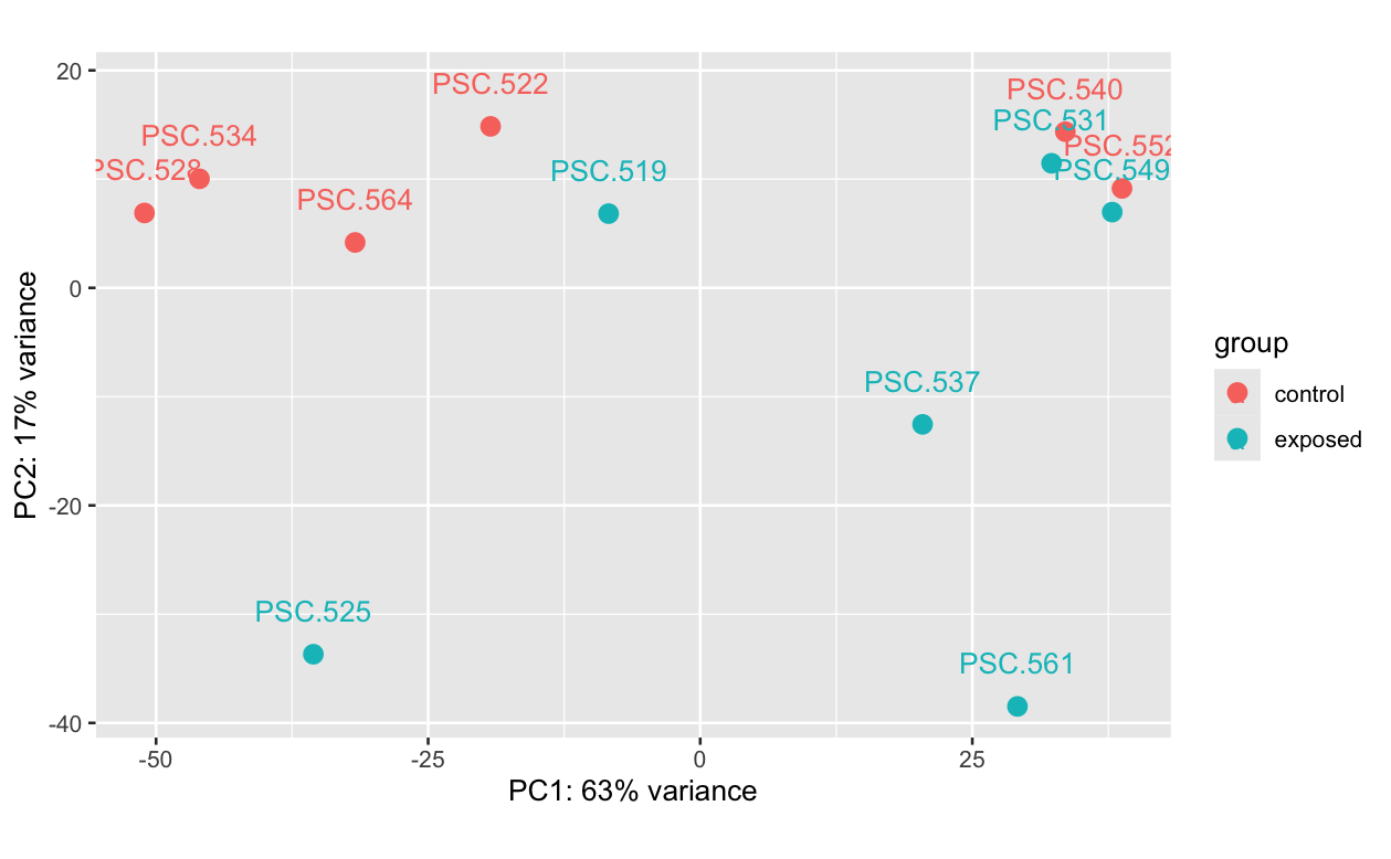
Figure 1. PCA plot of the variance transformed data
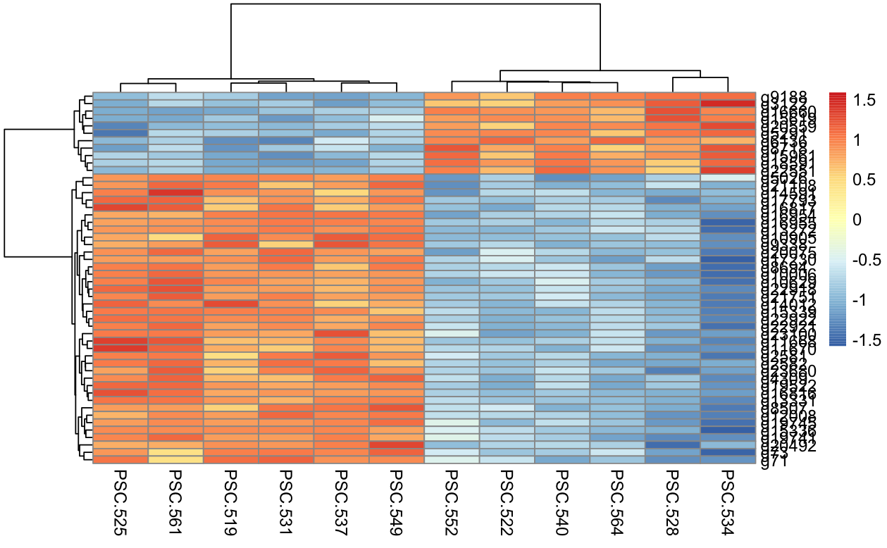
Figure 2. Heatmap of the top 50 DEGs from the Day 12 comparison between SSWD-exposed and control P. helianthoides. Orange/red are higher expression and pale blues and blue are lower expression.
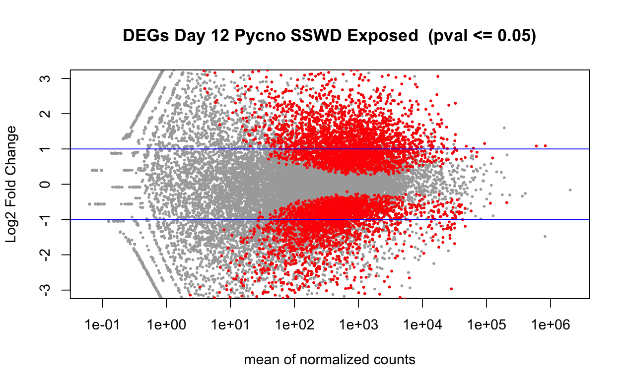
Figure 3. Volcano plot of the 5,686 DEGs from the comparison of Day 12 SSWD-exposed and control P. helianthoides.
Enrichment using topGO
For this process, I used a variety of resources. Steven ran some enrichment with topGO using Claude a while back and I looked through his code, and tried it myself in 39-topGO-enrichment.Rmd.
I also read through a bunch of online resources:
https://bioconductor.org/packages/release/bioc/vignettes/topGO/inst/doc/topGO_manual.R
https://bioc.r-universe.dev/articles/topGO/topGO_manual.html
https://nbisweden.github.io/workshop-RNAseq/1906/lab_functional.html
https://bioconductor.posit.co/packages/3.24/bioc/vignettes/topGO/inst/doc/topGO_manual.html
And on 2026-10-28 I met with Ariana who has done work with topGO and got help from her and her code.
Essentially, what the code does is:
- make a gene universe for the background using the gene IDs from the P. helianthoides gene count matrix.
- Create a vector for every gene for both the background and the gene list (DEGs):
pyc.geneList
0 1
17778 5686
- Create a GO ID map of the background (the annotated gene count matrix)
- Create a
topGOobject:pyc.GOdata <- new( "topGOdata", ontology = "BP", allGenes = pyc.geneList, # degs nodeSize = 5, #can comment out, but it removes spurious categories - trims out stuff with lower confidence in and core answer shuoldn't change geneSelectionFun = function(x) x, annot = annFUN.gene2GO, # for whole universe gene2GO = pyc.geneID2GO #for all the gene universe annotation )
numSigGenes(pyc.GOdata)
sum(feasible(pyc.GOdata))
telling number of gene is significant out of all feasible genes
first should be smaller than second number
[1] 2516
[1] 7490
Run enrichment:
pyc.resultFis <- runTest(
    pyc.GOdata,
    algorithm = "weight01",
    statistic = "fisher"
)
Results in a table of 5,757 rows: output/43-pycno-D12-DESeq2-topGO/pycno.D12.topGO_ALL_BP_results_nodeSize5.csv
Run a p-value adjustment:
From Ariana’s code:
allRes$bh_adjust_weight <- p.adjust(allRes$weightFisher, method=”BH”) #add adjusted p-values
BH is the benjamini hochberg correction
pyc.results.all$bh_adjust_weight <- p.adjust(pyc.results.all$Fisher, method="BH")
output/43-pycno-D12-DESeq2-topGO/pycno.D12.topGO_ALL_BP_results_BHpval_nodeSize5.csv
next, subset the results with padj < 0.05
p05_res <- pyc.results.all %>% dplyr::filter(Fisher < 0.05)
when using the nodeSize = 5, it’s a list of 260 rows
#BiocManager::install("org.Ce.eg.db")
library(rrvgo)

#Reduce/collapse GO term set with the rrvgo package
simMatrix <- calculateSimMatrix(p05_res$GO.ID,
                                orgdb="org.Ce.eg.db", #c. elegans database
                                ont="BP",
                                method="Rel")
 #calculate similarity
scores <- setNames(-log(as.numeric(p05_res$Fisher)), p05_res$GO.ID)
reducedTerms <- reduceSimMatrix(simMatrix,
                                scores,
                                threshold=0.7,
                                orgdb="org.Ce.eg.db")
dim(reducedTerms)
[1] 177 10
#keep only the goterms from the reduced list
p05_res_reduced <- p05_res %>%
  filter(GO.ID %in% reducedTerms$go)

#add in parent terms to list of go terms
p05_res_reduced$ParentTerm <- reducedTerms$parentTerm[match(p05_res_reduced$GO.ID, reducedTerms$go)]

length(unique(p05_res_reduced$ParentTerm))

p05_res_reduced <- p05_res_reduced %>% group_by(ParentTerm) %>% mutate("N_in_Parent" = dplyr::n()) %>% ungroup()
length(unique(p05_res_reduced$ParentTerm))
[1] 47
[1] 47
output/43-pycno-D12-DESeq2-topGO/p05_reduced_GO_and_parent.csv
Visualizations of enrichement using rrvgo
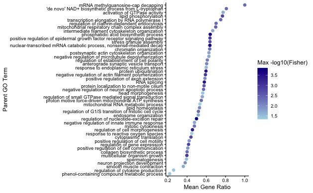
Figure 4. Enriched Biological gene ontology terms for P. helianthoides at day 12 comparing SSWD-exposed to control. The x-axis is the mean gene ratio, which is the number of DEGs annotated divided by the total number of genes from the gene count matrix annotated with that term. The color is that the darker blue, the more significant the Fisher p-value.
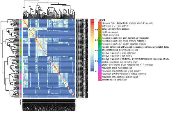
Figure 5. Similarity matrix heatmap of Day 12 enrichment for P. helianthoides. The threshold was set to 0.9.
From rrvgo vignette:
“rrvgo uses the similarity between pairs of terms to compute a distance matrix, defined as (1-simMatrix). The terms are then hierarchically clustered using complete linkage, and the tree is cut at the desired threshold, picking the term with the highest score as the representative of each group.
Therefore, higher thresholds lead to fewer groups, and the threshold should be read as the minimum similarity between group representatives.”
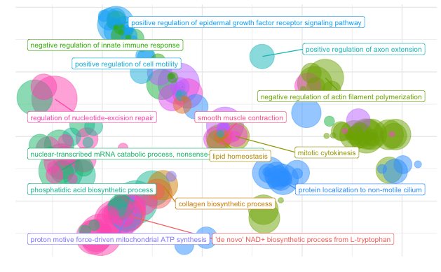
Figure 6. Bubble plot of enriched terms for P. helianthoides at Day 12… not super helpful to look at.
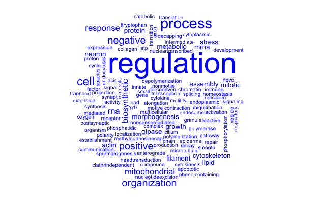
Figure 7. Word cloud of terms that appear frequently in the enriched Biological Processes from P. helianthoides at Day 12.
Notes from rrvgo vignette: “Word clouds are visualizations which reproduce a text putting emphasis to words which appear frequently in a text. They can help to identify processes and functions that happen more commonly in a set of enriched GO terms, as well as comparing between different sets.””
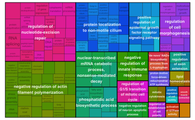
Figure 8. Treemap of P. helianthoides day 12 enrichment.
Notes/Questions:
- I did not remove low-count genes from the gene matrix before running
DESeq2–> should I? - For Fig. 4 –> would it be better if it’s the Benjamini-Hochberg correct p-value shown instead of the Fisher p-value?
Next steps:
- go over code again and make sure it all makes sense
- make other figures/result summaries
- put into paper and start discussing results